#The question
Every testing program implicitly trades money for a shorter exposure window: the time between an exploitable weakness appearing in your environment and that weakness being closed. Attackers are racing the same clock from the other side. If they find and use the weakness before you close it, the test schedule did not matter.
That framing gives a clean quantity to compute: the probability that an exposure is exploited before it is closed, as a function of how often you test, how reliably each test finds the exposure, how long fixes take, and how fast attackers are. The point of the model is not the absolute numbers — your parameters will differ — but the shape: which lever moves risk, and by how much.
#The model
We model a single exploitable exposure. Four random times matter, all measured in days from the moment it appears:
- : time until a test detects it.
- : time from detection to a verified fix. We take .
- : time until an attacker finds and exploits it, , independent of the defender.
- The exposure is closed at . It is exploited first if .
Because is exponential, the probability of exploitation before closure has a convenient form in terms of Laplace transforms:
For an exponential fix time the second factor is .
Periodic testing
Tests run every days. The exposure appears at a uniformly random point in the cycle, so the wait for the next test is . Each test independently finds a live exposure with probability — coverage is never perfect, because scope is sampled and testers run out of hours. If the first test misses, the next chance is days later, so with . Taking the transform:
and the mean exposure window is
The middle term is the one people forget: a test that misses a weakness doesn't just delay detection by a few days, it pushes it out by a full cycle.
Continuous testing
Continuous testing replaces the schedule with a detection delay , giving and therefore
#Parameters and why we chose them
We use per test, a fix time of days, and day for continuous detection. For attacker speed we bracket with three values taken from Mandiant's time-to-exploit analysis: an average of 63 days in 2018–2019, 32 days in 2021–2022 and 5 days in 2023 (the 2023 figure excludes outliers; with them the average is 47 days) [1]. Those are times from public disclosure to exploitation in the wild, not times for an attacker to find a weakness in your estate, so read as a scale for "how fast is the adversary you worry about", not as a measured constant.
We computed every value in closed form and checked it with a 400,000-trial Monte Carlo simulation per cell. The largest absolute difference between the two across all cells was 0.0007. Code and outputs are in the project's research/ directory.
#Results
| Testing regime | Mean exposure window | P(exploited), τ = 5 d | τ = 32 d | τ = 63 d |
|---|---|---|---|---|
| Annual | 287.8 days | 99.7% | 95.1% | 88.7% |
| Semi-annual | 150.9 days | 99.4% | 90.3% | 78.4% |
| Quarterly | 82.4 days | 98.8% | 81.4% | 63.7% |
| Monthly | 36.8 days | 96.5% | 61.1% | 40.8% |
| Weekly | 19.3 days | 88.1% | 40.4% | 24.5% |
| Continuous (d = 1 day) | 15.0 days | 78.1% | 32.5% | 19.5% |
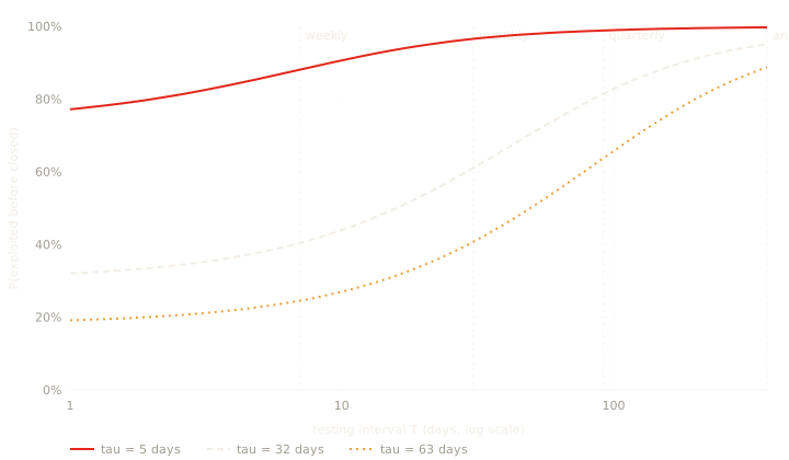
Three things stand out.
Annual testing is close to irrelevant against a fast adversary. With a 365-day cycle and 80% detection, the mean exposure window is 288 days. Against days, 95% of exposures are exploited before closure. The annual test is still useful for compliance and for finding long-lived structural problems, but as a control on time-sensitive exposure it does very little.
Moving from annual to monthly roughly halves risk at and cuts it by a third at . That's real, and it is why PTaaS and quarterly programs exist. But at even weekly testing leaves 88% of exposures exploited.
Once detection is continuous, the fix time is the whole game. Continuous detection at day with a 14-day fix still leaves 78% exploited at . The detection term has shrunk to almost nothing; what remains is .
#Sensitivity: fix time under continuous testing
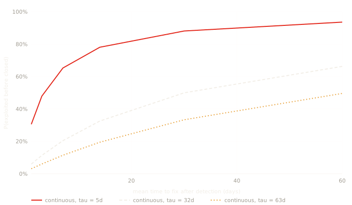
| Mean fix time r | Continuous, τ = 5 d | τ = 32 d | τ = 63 d | Annual (same r), τ = 32 d |
|---|---|---|---|---|
| 1 days | 30.6% | 6.0% | 3.1% | 93.2% |
| 3 days | 47.9% | 11.3% | 6.0% | 93.6% |
| 7 days | 65.3% | 20.4% | 11.4% | 94.2% |
| 14 days | 78.1% | 32.5% | 19.5% | 95.1% |
| 30 days | 88.1% | 50.0% | 33.3% | 96.4% |
| 60 days | 93.6% | 66.3% | 49.6% | 97.6% |
Under annual testing, fix time barely matters: the exposure window is dominated by waiting for the test. Under continuous testing, cutting mean fix time from 14 to 3 days at drops risk from 32.5% to 11.3%. This is the quantitative version of a familiar complaint: buying detection without buying remediation capacity moves the bottleneck, it doesn't remove it.
A useful rule of thumb falls out of the formula. When and , a first-order expansion gives
Risk is roughly linear in the total exposure time over the attacker's time scale. Halving fix time is worth exactly as much as halving detection delay — and fix time is usually the bigger number.
#What this means in practice
- Measure your . Seed known weaknesses (or use last year's findings that were reintroduced) and see how often your tests find them. A program with on a quarterly cycle has the same mean detection wait as one with on a half-yearly cycle.
- Track as a first-class metric. Time from proven finding to verified fix — not to ticket closure, to verified fix — is the number this model says you should obsess over once testing is continuous.
- Retest automatically. Without a retest, silently includes every fix that didn't actually work. The model treats a failed fix as an exposure that never closed.
- Use continuous testing to buy back fix time, not just detection. Proof of exploit and a minimal fix recommendation shorten directly; a list of scanner output does not.
#Run it on your own numbers
The model is four parameters and two lines of code. Plug in your own estimates — even rough ones — before arguing about test frequency:
from math import exp

def p_exploit_periodic(T, q, r, tau):
    a = exp(-T / tau)
    lap_w = (tau / T) * (1 - a) * q / (1 - (1 - q) * a)
    return 1 - lap_w / (1 + r / tau)

def p_exploit_continuous(d, r, tau):
    return 1 - 1 / ((1 + d / tau) * (1 + r / tau))

# quarterly tests that find 60% of issues, 21-day fixes, a 30-day adversary
print(p_exploit_periodic(91, 0.6, 21, 30))   # 0.887
print(p_exploit_continuous(1, 21, 30))       # 0.43
Three estimates do most of the work. : the share of known-bad conditions your tests actually find — measure it by checking how many of last cycle's findings the next test re-discovered after they regressed. : median days from a proven finding to a verified fix, by severity. : pick the adversary you're defending against; for internet-facing systems the public time-to-exploit data argues for days, not months.
The output is a probability per exposure. Multiply by the number of exploitable exposures you expect per year — your historical findings rate is a reasonable proxy — and you have an expected count of exposures that were open long enough to be used. That is the number to put next to the testing budget.
#Limitations
This is a single-exposure model. It ignores dependence between exposures (one exposure often enables another; see our attack-path study), assumes attackers are memoryless (exponential ), and treats detection probability per test as constant. Real fix times are heavier-tailed than exponential; a lognormal with the same mean raises risk further because the long tail of slow fixes dominates. The attacker-speed values are anchors from public exploitation data, not measurements of attackers targeting any particular organization. None of these change the qualitative conclusions, but all of them change the numbers.
#Frequently asked questions
How often should a penetration test be performed?
Most standards require at least annually and after significant change. The exposure-window model shows annual testing does little against fast attackers: with an 80% detection rate, about 95% of exposures would be exploited before closure if attackers take a month on average. Continuous testing plus fast remediation is what moves the number.
Is continuous penetration testing worth it if we can't fix things faster?
Partly. Continuous detection removes the waiting time for the next test, but once detection is fast, risk is driven by mean time to fix. Under our model, risk is roughly (detection delay + fix time) divided by attacker time scale.
#Sources
- [1] Mandiant (Google Cloud), “How Low Can You Go? An Analysis of 2023 Time-to-Exploit Trends,” 2024
- [2] PCI Security Standards Council, FAQ on penetration and segmentation testing frequency for service providers
Shrink d and r at the same time.
Rogue detects continuously and ships each finding with proof and the smallest fix, then retests on merge. We'll measure your current q and r in a ten-day sprint.
Book a briefing